General description of the globalICP method

The Iterative Closest Point (ICP) algorithm (Chen & Medioni (1991), Besl & McKay (1992)) improves the alignment of two (or more) point clouds by minimizing iteratively the discrepancies within the overlap area of these point clouds. Nowadays the term ICP does not necessarily refer to the algorithm presented in the original publications, but rather to a group of surface matching algorithms which have in common the following aspects:

• I: correspondences are established iteratively (i.e. not only once)
• C: as correspondence the closest point, or more generally, the corresponding point, is used
• P: correspondences are established on a point basis (instead of using e.g. interpolated surfaces or rasters)

The following flow diagram illustrates the functionality of this module. The main iteration loop consists of 7 main steps, which are described below.

Figure 1: Functionality of globalICP.

In the simplest case, the ICP algorithm is used to improve the orientation of a single loose point cloud with respect to a single fixed point cloud. The main steps of the algorithm are explained on the basis of this case. The initial orientation of the two point clouds is visualized in Figure 2. As can be seen, the point clouds are already roughly aligned, which is a main requirement of the ICP algorithm.

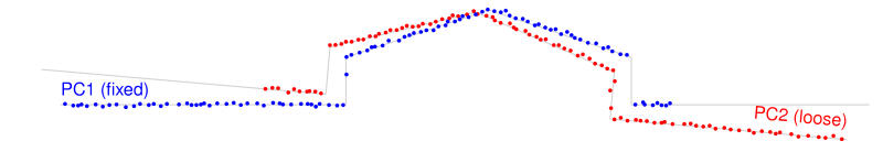
Figure 2: Initial state of the point clouds.

Step 1 - Find overlap: The overlap area of the point clouds is determined by using so-called voxel hulls. Voxel hulls are a low resolution representation of the volume occupied by a point cloud. For the computation of the voxel hull the object space is subdivided into a voxel structure. The voxel hull of a point cloud consists of all voxels which contain at least one point of the point cloud. The parameter HullVoxelSize defines the edge length of a single voxel.

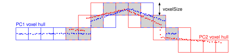
Figure 3: Overlap area of the point clouds (grey filled voxels) as intersection of the two voxel hulls (blue resp. red voxels).

Step 2 - Selection: A subset of points is selected within the overlap area in one point cloud. For this, points are first selected uniformly in object space, which leads to a homogeneous distribution of the points within the overlap area (uniform sampling). The mean sampling distance in each coordinate direction is defined by the parameter UniformSamplingDistance. The selected subset of points can be further refined with the strategies normal space sampling or maximum leverage sampling, which are described in Advanced selection strategies for correspondences.

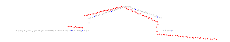
Figure 4: Selection of points in first point cloud.

Step 3 - Matching: Find the closest points (= nearest neighbors) of the selected subset in the other point cloud. This step leads to a set of correspondences which possibly also includes some outliers.

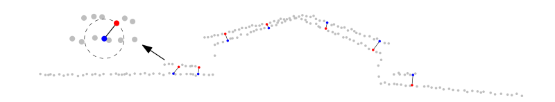
Figure 5: Matching of the selected points (blue / from previous step) to the closest points (red) in the second point cloud.

Step 4 - Rejection: Rejection of false correspondences (outliers) based on the compatibility of points. Correspondences are rejected if:

• the euclidean distance between corresponding points is larger than the value specified by the parameter MaxDistance.
• the roughness attribute of one of the corresponding points is larger than the value specified by the parameter MaxRoughness. (Note: as roughness attribute the standard deviation in normal direction of the points used for plane fitting is used.)
• the angle between the normals of corresponding points is larger than the value specified by the parameter MaxDeltaAngle.

Since it is not guaranteed that with these strategies all outliers are rejected, a robust adjustment method is used in step 6 (Minimization) for the detection and deactivation of the remaining ones.

Step 5 - Weighting: In this step a weight between 0 and 1 is assigned to each correspondence. Weights are based on:

• the roughness attribute of corresponding points
• the angle between the normals of corresponding points.

Step 6 - Minimization: Estimation of the transformation parameters (for the loose point cloud) by a least squares adjustment. The adjustment minimizes the sum of squared point-to-plane distances. The point-to-plane distance of two corresponding points is defined as the orthogonal distance of one point to the fitted plane of the other point.

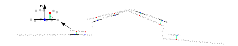
Figure 6: Minimization of the point-to-plane distances (green) between corresponding points.

Step 7 - Transformation: Transformation of the loose point cloud with the estimated parameters. The transformation model can be chosen with the parameter NoOfTransfParam.

After step 7, a convergence criterion is tested. If it is not met, the process restarts with a new iteration from step 1 (Figure 1). However, if subsets are defined by the parameter SubsetRadius, the iteration loop restarts from step 3 and the first two steps are only performed once. The total number of iterations heavily depends on the initial orientation of the points clouds, but typically, between 3 and 10 iterations should be sufficient to reach the global minimum.

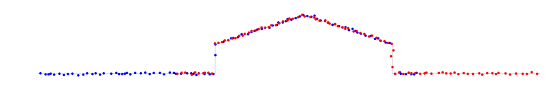
Figure 7: Final state of the point clouds.

Note that the globalICP class is not restricted to two point clouds, but can handle an arbitrary number of point clouds simultaneously.

Literature

Besl, P. J., McKay, N. D. (1992): Method for registration of 3-d shapes. In: Robotics-DL tentative, International Society for Optics and Photonics, pp. 586-606.

Chen, Y., Medioni, G. (1991): Object modelling by registration of multiple range images. Image and Vision Computing 10(3), pp. 145-155. Range Image Understanding.