INTRO: WORKING WITH THE POINTCLOUD CLASS IN MATLAB
This document demonstrates the basic usage of the pointCloud class on the basis of 10 short tutorials .
Contents
- Where to get help
- (1) Import of a point cloud WITHOUT attributes and visualize it
- (2) Import a point cloud WITH point attributes and visualize one of them
- (3) Import a point cloud from a matrix
- (4) RGB-colored plot of a point cloud
- (5) Import two point clouds and visualize them in different colors
- (6) Select a subset of points (i.e. filter/thin out point cloud) and export them to a text file
- (7) Calculate normals of a point cloud and visualize them
- (8) Transform a point cloud
- (9) Save and load point cloud
- (10) Create a copy of an object and select a subset of points in it
Note: You can extract the code from this html file with the matlab function grabcode
Where to get help
Before starting, a short hint on how to access the helpscreen of the methods (=functions) used within this tutorial:
% Help for the constuctor method (for object creation)
help pointCloud.pointCloud  % Import of point cloud data.

% Help for regular methods (to apply on the objects properties (=data))
help pointCloud.select      % Select a subset of points.
help pointCloud.plot        % Plot of point cloud.
help pointCloud.normals     % Compute normal vectors of activated points.
help pointCloud.plotNormals % Plot normal vectors of point cloud in 3d.
help pointCloud.info        % Report informations about the point cloud to the command window.
help pointCloud.transform   % Coordinate transformation of point cloud.
help pointCloud.export      % Export activated points to a file.
help pointCloud.save        % Save point cloud object as mat file.
help pointCloud.reconstruct % Reconstruct object only with active points.
help pointCloud.copy        % Create an indipendent copy of a point cloud object.
(1) Import of a point cloud WITHOUT attributes and visualize it
clc; clear; close; % clear everything

% Import a point cloud from a plain text file (run type('Lion.xyz') to see the contents of the file)
pc = pointCloud('Lion.xyz');

% Generate a z-colored view of the point cloud
pc.plot;

% Set three-dimensional view and add title
view(3); title('Z-colored plot of point cloud', 'Color', 'w');

Remember:
- Each method of the pointCloud class (e.g. pc.plot) generates a workspace output .
- Point coordinates x,y,z are saved in the object attribute pc.X
- An information about the point cloud can be displayed with the method pc.info
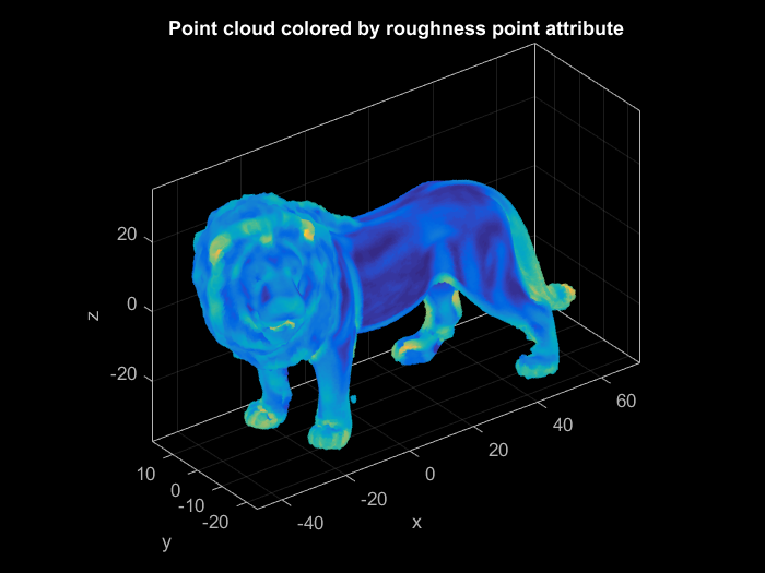
(2) Import a point cloud WITH point attributes and visualize one of them
clc; clear; close; % clear everything

% Import point cloud with attributes (nx, ny, nz are the components of the normal vectors)
pc = pointCloud('Lion.xyz', 'Attributes', {'nx' 'ny' 'nz' 'roughness'});

% Plot point cloud colored according to imported attribute 'roughness'
pc.plot('Color', 'A.roughness', ... % attribute to plot
        'MarkerSize', 5); % size of points

% Set three-dimensional view and add title
view(3); title('Point cloud colored by roughness point attribute', 'Color', 'w');
Remember:
- Point attributes are saved in the object attribute pc.A
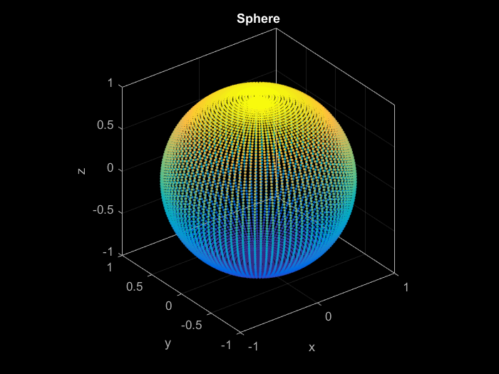
(3) Import a point cloud from a matrix
clc; clear; close; % clear everything

% Generate points on a unit sphere
[x, y, z] = sphere(100);
x = x(:); y = y(:); z = z(:);

% Import points and define a label for the point cloud
pc = pointCloud([x y z], 'Label', 'sphere');

% Plot point cloud
pc.plot('MarkerSize', 5);

% Set three-dimensional view and add title
view(3); title('Sphere', 'Color', 'w');
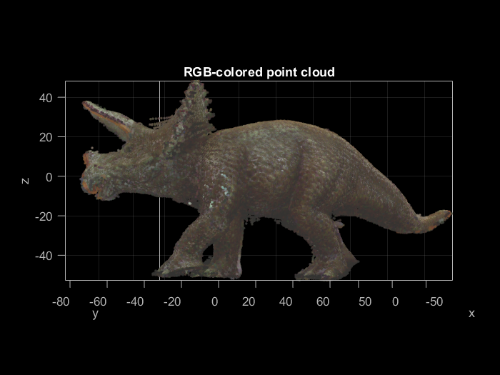
(4) RGB-colored plot of a point cloud
clc; clear; close; % clear everything

% Import point cloud with attributes red, green and blue
pc = pointCloud('Dino.xyz', 'Attributes', {'r' 'g' 'b'});

% Plot point cloud
pc.plot('Color', 'A.rgb', ... % rgb-colored plot
        'MarkerSize', 5); % size of points

% Set three-dimensional view and add title
view(110,0); title('RGB-colored point cloud', 'Color', 'w');
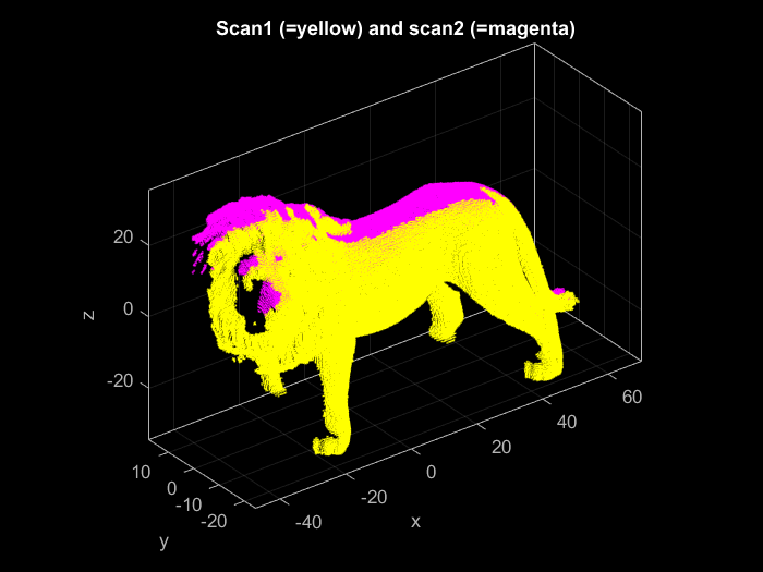
(5) Import two point clouds and visualize them in different colors
clc; clear; close; % clear everything

% Import point clouds
scan1 = pointCloud('LionScan1.xyz');
scan2 = pointCloud('LionScan2.xyz');

% Plot
scan1.plot('Color', 'y'); % yellow
scan2.plot('Color', 'm'); % magenta

% Set three-dimensional view and add title
view(3); title('Scan1 (=yellow) and scan2 (=magenta)', 'Color', 'w');
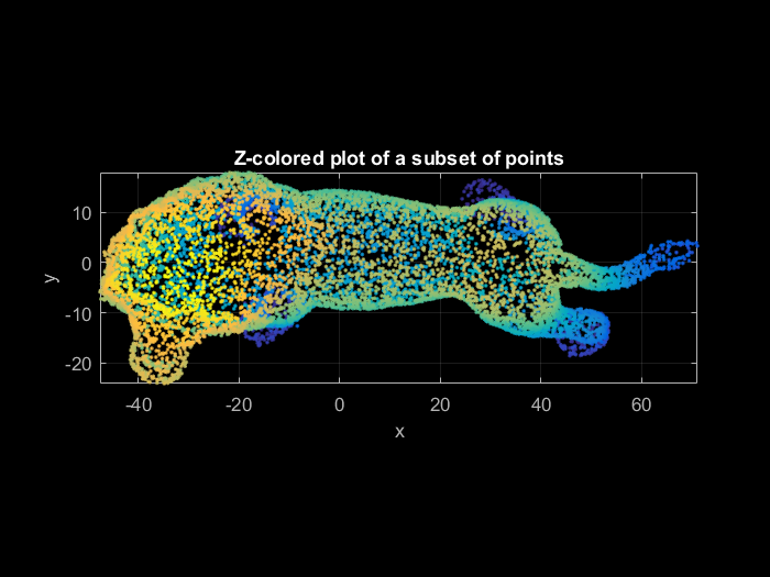
(6) Select a subset of points (i.e. filter/thin out point cloud) and export them to a text file
clc; clear; close; % clear everything

% Import point cloud
pc = pointCloud('Lion.xyz', 'Attributes', {'nx' 'ny' 'nz' 'roughness'});

% Select a random subset of points
pc.select('RandomSampling', 5); % select randomly 5 percent of points

% Export selected points to a plain text file with attributes
pc.export('LionSubset.xyz', 'Attributes', {'nx' 'ny' 'nz' 'roughness'});

% Plot
pc.plot('MarkerSize', 5);

% Set title
title('Z-colored plot of a subset of points', 'Color', 'w');
Remember:
- The attribute pc.act is a n-by-1 logical vector defining for each point if it is active (true) or not active (false) .
- Most methods apply only on active points .
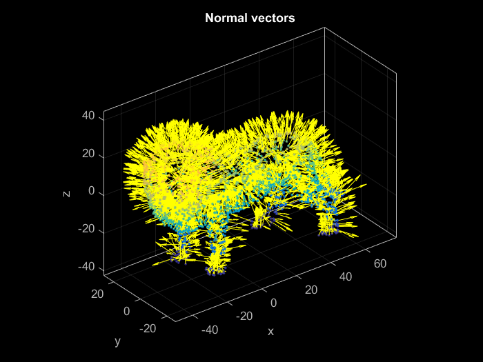
(7) Calculate normals of a point cloud and visualize them
clc; clear; close; % clear everything

% Import point cloud
pc = pointCloud('Lion.xyz');

% Select a random subset of points
pc.select('RandomSampling', 1); % select randomly 1 percent of points

% Calculate normals (normals are only calculated for the selected points)
pc.normals(2); % search radius is 2

% Plot point cloud and normals
pc.plot('MarkerSize', 5);
pc.plotNormals('Scale', 10, 'Color', 'y'); % lenght of normals is 10

% Set three-dimensional view and add title
view(3); title('Normal vectors', 'Color', 'w');
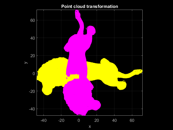
(8) Transform a point cloud
clc; clear; close; % clear everything

% Import point cloud
pc = pointCloud('Lion.xyz');

% Plot original point cloud
pc.plot('Color', 'y');

% Transformation with a rotation angle of 100 gradians about the z axis
pc.transform(1, opk2R(0, 0, 100), zeros(3,1)); % opk2R generates a rotation matrix from 3 rotation angles (about the x, y and z axis / units = gradian!)

% Plot transformed point cloud
pc.plot('Color', 'm'); title('Point cloud transformation', 'Color', 'w');
Remember:
- The transformation model used in this method is:
 (for more information run help pointCloud.transform)
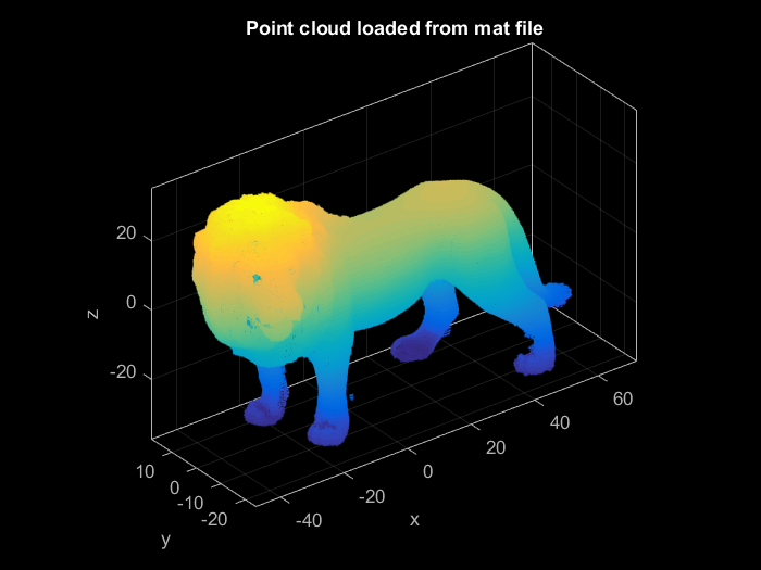
(9) Save and load point cloud
clc; clear; close; % clear everything

% Import point cloud
pc = pointCloud('Lion.xyz');

% Save to mat file
pc.save('Lion.mat');

% Clear point cloud
clear pc;

% Load point cloud from mat file
pcLoaded = pointCloud('Lion.mat');

% Plot
pcLoaded.plot;

% Set three-dimensional view and add title
view(3); title('Point cloud loaded from mat file', 'Color', 'w');
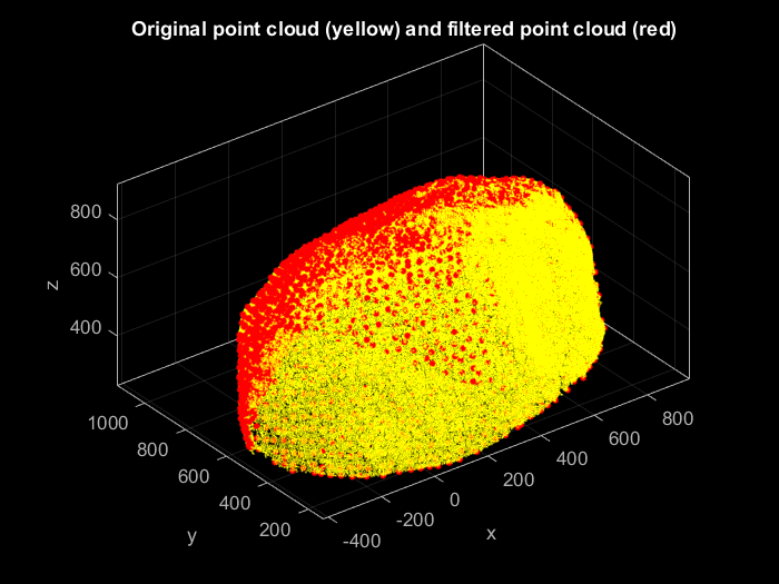
(10) Create a copy of an object and select a subset of points in it
clc; clear; close; % clear everything

% Import point cloud
pc = pointCloud('Stone.ply'); % attributes from ply file are imported automatically

% Create an indipendent copy of the object
pcCopy = pc.copy;

% Select a subset of points and remove all non active points
pcCopy.select('UniformSampling', 40); % uniform sampling with mean sampling distance of 40 mm
pcCopy.reconstruct;

% Plot both point clouds
pc.plot('Color', 'y', 'MarkerSize', 1);
pcCopy.plot('Color', 'r', 'MarkerSize', 10);
view(3); title('Original point cloud (yellow) and filtered point cloud (red)', 'Color', 'w');